확률론3-2 : 나이브 베이즈(Naive Bayes)분류기 [in r]

베이즈정리를 모르신다면 아래의 글을 보시길 권장합니다.https://pastryofjsmath.tistory.com/11

확률론3 - 베이즈정리(Bayes Theorem)

 

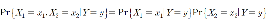
나이브 베이즈 분류기는 입력변수 간 서로 독림임을 가정으로 시작합니다

조건부 확률의 조건부 독립이 성립해야 합니다.

 

 

조건부 독립(Conditional Independence)

분류모델 성능 측정으로 매우 유명한 타이타닉 데이터 셋으로 해보겠습니다.

titanic.RData

0.01MB

 

제일 먼저, 나이브 베이즈 사용을 위한 패키지를 라이브러리를 해주어야합니다.

install.packages("e1071")
library("e1071")
#titanic<-read.csv()

 

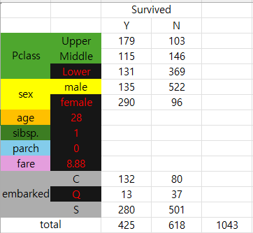
> titanic %>% summary()
    pclass    survived      sex                 age         
 Upper :282   No :618   Length:1043        Min.   : 0.1667  
 Middle:261   Yes:425   Class :character   1st Qu.:21.0000  
 Lower :500             Mode  :character   Median :28.0000  
                                           Mean   :29.8132  
                                           3rd Qu.:39.0000  
                                           Max.   :80.0000  
     sibsp            parch             fare        embarked
 Min.   :0.0000   Min.   :0.0000   Min.   :  0.00   ?:  0   
 1st Qu.:0.0000   1st Qu.:0.0000   1st Qu.:  8.05   C:212   
 Median :0.0000   Median :0.0000   Median : 15.75   Q: 50   
 Mean   :0.5043   Mean   :0.4219   Mean   : 36.60   S:781   
 3rd Qu.:1.0000   3rd Qu.:1.0000   3rd Qu.: 35.08           
 Max.   :8.0000   Max.   :6.0000   Max.   :512.33
 
 > titanic %>% str()
'data.frame':	1043 obs. of  8 variables:
 $ pclass  : Factor w/ 3 levels "Upper","Middle",..: 3 3 2 3 3 2 3 2 1 3 ...
 $ survived: Factor w/ 2 levels "No","Yes": 1 1 1 1 1 1 1 2 2 1 ...
 $ sex     : chr  "male" "male" "male" "female" ...
 $ age     : num  17 30 23 30 29 29 16 36 30 19 ...
 $ sibsp   : int  0 0 0 0 0 1 0 1 0 0 ...
 $ parch   : int  0 0 0 0 0 0 0 0 0 0 ...
 $ fare    : num  7.9 7.22 15.05 8.66 7.92 ...
 $ embarked: Factor w/ 4 levels "?","C","Q","S": 4 2 2 4 4 2 4 4 2 4 ...

우선  pclass='Lower', sex='female', age=28, sibsp=1, parch=0, fare= 8.88, embarked='Q'인 사람 한명이 탔다고 합니다.

그리고 이 사람의 생존유무를 체크한다고 합시다.

그렇다면 아래와 같이 쓸 수 있습니다.

생존여부에 따른 조건부확률

 

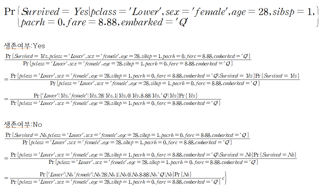
위의 굵은 글씨는 어떠한 사람이라는 가정하에 생존할 확률을 뜻합니다.

다음줄은 등식을 알고 있어야합니다.

조건부 확률

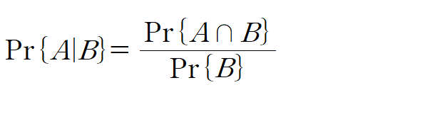
하나씩 보자면 생존여부:Yes 라는 첫줄에서는 위의 등식을 만족합니다 (콤마(,):and,교집합이란 뜻입니다.)

그리고 다음줄은 분자를 생존여부에 따른 조건부 확률을  생존을 가정하에 어떤 사람일 확률로 변형한 모습입니다.

마지막 줄은 조건부 독립이란 성질에 의해 각각의 조건부확률로 바뀐 모습입니다. 이를 생존여부:No인 경우에도 해주어서 각 확률을 비교하여 큰 쪽으로 분류하는 것이 나이브 베이즈 분류기입니다.

 

nb2 <- naiveBayes(survived ~. , data=titanic_train)
> titanic_test2 <- data.frame(pclass='Lower',sex='female',
+                             age=28,sibsp=1,parch=0,
+                             fare= 8.88,embarked='Q')
> predict(nb2,titanic_test2)
[1] No
Levels: No Yes

#얼만큼의 확률이 나왔길래 No가 나왔는가?
> predict(nb2,titanic_test2,type='raw')
            No       Yes
[1,] 0.7049402 0.2950598

 

#전체 데이터프레임에서의 샘플링을 통한 train/test
sam<-sample(x = 1:1043,size = 800,replace = F)
sam %>% head()
titanic_train <- titanic[sam,]
titanic_test <- titanic[-sam,]

nb2 <- naiveBayes(survived ~. , data=titanic_train)
titanic_test$pred <-predict(nb2,titanic_test[,-2])

#정확도
(titanic_test$survived == titanic_test$pred) %>% mean()
[1] 0.8024691

 

아래는 다른 예제를 준비해봤습니다.

 

https://www.kaggle.com/datasets/uciml/mushroom-classification/data

Mushroom Classification

cap-shape(갓 모양)

bell:b.종모양, conical:c.원뿔,convex:x.볼록,flat:f.평평,knobbed:k.돌기?같은 것을 말하는 것같습니다.

sunnken:s.안으로 파인 모양

 

cap-surface(갓 표면)

fibrous:f.섬유, grooves:g.홈이 있는 표면, scaly:y.비늘표면,smooth=s.부드러움

 

cap-color(갓 색깔)

brown:n, buff:b.누런색, cinnamon:c.시나몬색 gray:g, green:r, pink=p,

purple:u, red:e, white:w, yellow:y

 

등등 위의 주소에 컬럼에 대한 설명이 있으니 궁금하신분들은 읽어보시길 바랍니다.

 

이에 대해 우리의 목표는  (classes: edible=e, poisonous=p)  식용,독인지를 분류하는 것이 목표입니다.

mushrooms<-read.csv('C:/Users/PJS/Documents/study/확률론/code/mushrooms.csv')
mushrooms %>% head()
mushrooms %>% str()
mushrooms %<>% mutate_all(as.factor) #모든 컬럼을 팩터로 변환

#stalk.root의 ?(결측치) 존재인식.####
#아예 제거.
mushrooms<-mushrooms %>% filter(mushrooms$stalk.root!='?')

#train/test 데이터 셋 분류
sam<-sample(1:nrow(mushrooms),size = nrow(mushrooms)*0.8,replace = F)
mushrooms_train <- mushrooms[sam,]
mushrooms_test <- mushrooms[-sam,]

#데이터셋에 있는 식용과 독의 비율은?
ggplot(data=mushrooms,aes(x=class))+
  geom_bar(color='purple',lwd=1.3)
  
> #e,p의 비율
> ((mushrooms$class=='p') %>% sum)/nrow(mushrooms)
[1] 0.3819986
> ((mushrooms$class=='e') %>% sum)/nrow(mushrooms)
[1] 0.6180014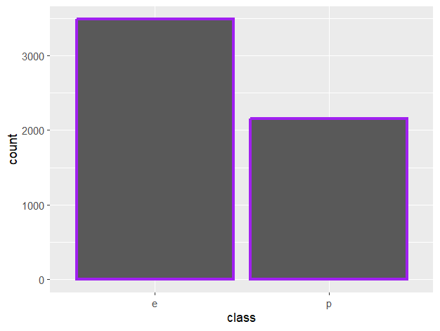

식용과 독의 비율

nb <- naiveBayes(class~ ., data = mushrooms_train)
mushrooms_test$pred <- predict(nb,mushrooms_test[,-1])
mushrooms_test %>% head()

#실제로 테스트 데이터마다 어떤 확률값으로 결정되었는가?
predict(nb,mushrooms_test[,-1],type='raw')
#정확도
(mushrooms_test$class == mushrooms_test$pred) %>% mean()
[1] 0.9486271

 

-출처: AI소프트웨어학과 이두호교수님 강의파일